List and load spectral bands
# list files from a directory library ("terra" )
Warning: package 'terra' was built under R version 4.3.2
= list.files ("clustering_data/data/task" , pattern = " \\ .TIF$" , full.names = TRUE )
[1] "clustering_data/data/task/LC08_L2SP_191023_20230605_20230613_02_T1_SR_B1.TIF"
[2] "clustering_data/data/task/LC08_L2SP_191023_20230605_20230613_02_T1_SR_B2.TIF"
[3] "clustering_data/data/task/LC08_L2SP_191023_20230605_20230613_02_T1_SR_B3.TIF"
[4] "clustering_data/data/task/LC08_L2SP_191023_20230605_20230613_02_T1_SR_B4.TIF"
[5] "clustering_data/data/task/LC08_L2SP_191023_20230605_20230613_02_T1_SR_B5.TIF"
[6] "clustering_data/data/task/LC08_L2SP_191023_20230605_20230613_02_T1_SR_B6.TIF"
[7] "clustering_data/data/task/LC08_L2SP_191023_20230605_20230613_02_T1_SR_B7.TIF"
#Display metadata # load raster data = rast (files)# calling the object displays the metadata
class       : SpatRaster
dimensions  : 1946, 2052, 7  (nrow, ncol, nlyr)
resolution  : 30, 30  (x, y)
extent      : 562455, 624015, 5797635, 5856015  (xmin, xmax, ymin, ymax)
coord. ref. : WGS 84 / UTM zone 33N (EPSG:32633)
sources     : LC08_L2SP_191023_20230605_20230613_02_T1_SR_B1.TIF
              LC08_L2SP_191023_20230605_20230613_02_T1_SR_B2.TIF
              LC08_L2SP_191023_20230605_20230613_02_T1_SR_B3.TIF
              ... and 4 more source(s)
names       : LC08_~SR_B1, LC08_~SR_B2, LC08_~SR_B3, LC08_~SR_B4, LC08_~SR_B5, LC08_~SR_B6, ...
min values  :           6,          21,        3531,        3123,        6811,        6857, ...
max values  :       36332,       34628,       36371,       37924,       42025,       60674, ...
shorten and rename spectral bands
names (landsat) # original names
[1] "LC08_L2SP_191023_20230605_20230613_02_T1_SR_B1"
[2] "LC08_L2SP_191023_20230605_20230613_02_T1_SR_B2"
[3] "LC08_L2SP_191023_20230605_20230613_02_T1_SR_B3"
[4] "LC08_L2SP_191023_20230605_20230613_02_T1_SR_B4"
[5] "LC08_L2SP_191023_20230605_20230613_02_T1_SR_B5"
[6] "LC08_L2SP_191023_20230605_20230613_02_T1_SR_B6"
[7] "LC08_L2SP_191023_20230605_20230613_02_T1_SR_B7"
names (landsat) = paste0 ("B" , 1 : 7 ) # shorten the names names (landsat) # new names
[1] "B1" "B2" "B3" "B4" "B5" "B6" "B7"
Load vector data and transform CRS
# load vector data = vect ("clustering_data/data/task/Szamotuly.gpkg" )
 class       : SpatVector
 geometry    : polygons
 dimensions  : 1, 0  (geometries, attributes)
 extent      : 16.01377, 16.74077, 52.37375, 52.79406  (xmin, xmax, ymin, ymax)
 source      : Szamotuly.gpkg
 coord. ref. : lon/lat ETRS89 (EPSG:4258)
= project (poly, "EPSG:32633" )crs (poly, describe = TRUE )$ code # check EPSG after transformation
Crop raster data to the area.
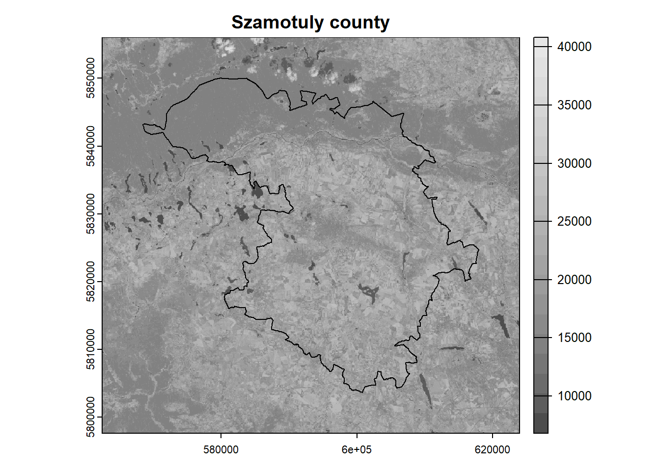
= gray.colors (n = 20 ) # define the color scheme plot (landsat[[5 ]], main = "Szamotuly county" , col = colors) # plot NIR band plot (poly, add = TRUE ) # add polygon
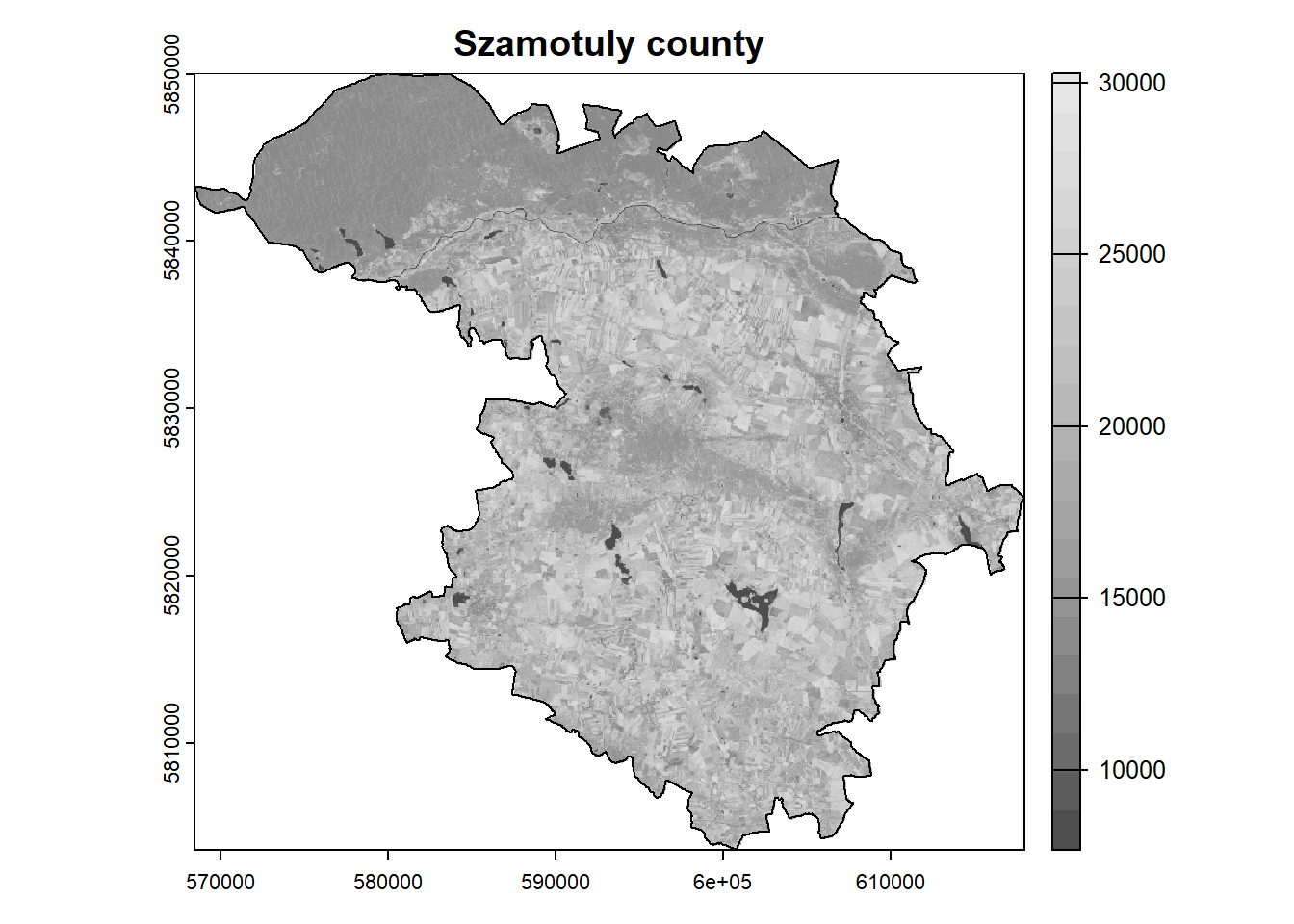
= crop (landsat, poly, mask = TRUE )plot (landsat[[5 ]], main = "Szamotuly county" , col = colors)plot (poly, add = TRUE ) Scale the values and remove outliers
Warning: [summary] used a sample
       B1              B2              B3              B4
 Min.   : 5944   Min.   : 2420   Min.   : 7609   Min.   : 6939
 1st Qu.: 7806   1st Qu.: 8046   1st Qu.: 8907   1st Qu.: 8441
 Median : 8009   Median : 8252   Median : 9401   Median : 8835
 Mean   : 8316   Mean   : 8613   Mean   : 9712   Mean   : 9452
 3rd Qu.: 8601   3rd Qu.: 8902   3rd Qu.:10108   3rd Qu.: 9958
 Max.   :19577   Max.   :20198   Max.   :21355   Max.   :22268
 NA's   :51153   NA's   :51152   NA's   :51151   NA's   :51151
       B5              B6              B7
 Min.   : 7692   Min.   : 7322   Min.   : 7326
 1st Qu.:15928   1st Qu.:11605   1st Qu.: 9348
 Median :19210   Median :12471   Median : 9948
 Mean   :19194   Mean   :13496   Mean   :11210
 3rd Qu.:22071   3rd Qu.:14844   3rd Qu.:12193
 Max.   :29478   Max.   :25647   Max.   :23481
 NA's   :51151   NA's   :51151   NA's   :51151
= landsat * 2.75e-05 - 0.2 summary (landsat)
Warning: [summary] used a sample
       B1              B2              B3              B4
 Min.   :-0.04   Min.   :-0.13   Min.   :0.01    Min.   :-0.01
 1st Qu.: 0.01   1st Qu.: 0.02   1st Qu.:0.04    1st Qu.: 0.03
 Median : 0.02   Median : 0.03   Median :0.06    Median : 0.04
 Mean   : 0.03   Mean   : 0.04   Mean   :0.07    Mean   : 0.06
 3rd Qu.: 0.04   3rd Qu.: 0.04   3rd Qu.:0.08    3rd Qu.: 0.07
 Max.   : 0.34   Max.   : 0.36   Max.   :0.39    Max.   : 0.41
 NA's   :51153   NA's   :51152   NA's   :51151   NA's   :51151
       B5              B6              B7
 Min.   :0.01    Min.   :0.00    Min.   :0.00
 1st Qu.:0.24    1st Qu.:0.12    1st Qu.:0.06
 Median :0.33    Median :0.14    Median :0.07
 Mean   :0.33    Mean   :0.17    Mean   :0.11
 3rd Qu.:0.41    3rd Qu.:0.21    3rd Qu.:0.14
 Max.   :0.61    Max.   :0.51    Max.   :0.45
 NA's   :51151   NA's   :51151   NA's   :51151
Prepare the matrix for classification (remove empty values and sample).
< 0 ] = NA > 1 ] = NA
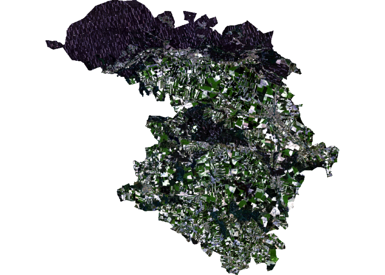
= plotRGB (landsat, r = 4 , g = 3 , b = 2 , scale = 1 , stretch = "lin" )
= values (landsat)nrow (mat) # print number of rows/pixels
= na.omit (mat)nrow (mat_omit)
set.seed (1 )= kmeans (mat_omit, centers = 5 )
          B1         B2         B3         B4        B5        B6         B7
1 0.02166975 0.02913068 0.05963210 0.04659851 0.3635857 0.1548141 0.08215531
2 0.04527543 0.05493472 0.08671713 0.09044609 0.2969842 0.2398647 0.17131855
3 0.07720274 0.09108228 0.13243481 0.15542923 0.3087454 0.3347357 0.29259717
4 0.01932286 0.02474700 0.04490836 0.03620496 0.2066564 0.1240278 0.06635903
5 0.01300182 0.02149046 0.05689401 0.03608233 0.4637850 0.1186973 0.05500941
head (mdl$ cluster) # display the first 6 elements Use the k-means algorithm for clustering and validate the results with the silhouette index. Check how the results change depending on the number of clusters. Optionally, you can test another clustering method .
set.seed (1 )# draw sample indexes = sample (1 : nrow (mat_omit), size = 10000 )head (idx)
[1] 452737 124413 856018 25173 640775 538191
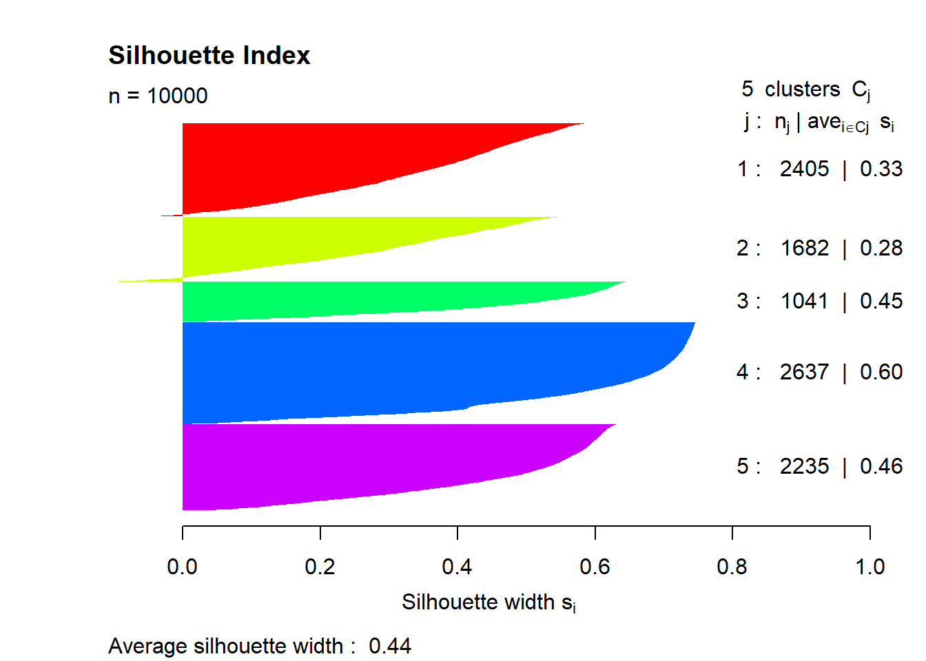
# calculate silhouette index = silhouette (mdl$ cluster[idx], dist (mat_omit[idx, ]))summary (sil)
Silhouette of 10000 units in 5 clusters from silhouette.default(x = mdl$cluster[idx], dist = dist(mat_omit[idx, ])) :
 Cluster sizes and average silhouette widths:
     2405      1682      1041      2637      2235
0.3322348 0.2783603 0.4524438 0.5989181 0.4629095
Individual silhouette widths:
   Min. 1st Qu.  Median    Mean 3rd Qu.    Max.
-0.1087  0.2861  0.4638  0.4352  0.5979  0.7465
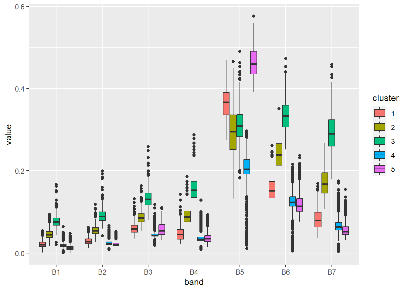
= rainbow (n = 5 )plot (sil, border = NA , col = colors, main = "Silhouette Index" ) Try to interpret what the clusters represent using a boxplot and RGB composition.
library ("tidyr" ) # data transformation
Warning: package 'tidyr' was built under R version 4.3.2
Attaching package: 'tidyr'
The following object is masked from 'package:terra':

    extract
library ("ggplot2" ) # data visualization
Warning: package 'ggplot2' was built under R version 4.3.2
= cbind (mat_omit[idx, ], cluster = mdl$ cluster[idx])= as.data.frame (stats)head (stats)
         B1        B2        B3        B4        B5        B6        B7 cluster
1 0.0163700 0.0229425 0.0522025 0.0380675 0.3392750 0.1368750 0.0792075       1
2 0.0336675 0.0361700 0.0493150 0.0464825 0.1752375 0.1334375 0.0773100       4
3 0.0161500 0.0264900 0.0623225 0.0539625 0.3488725 0.1362975 0.0748900       1
4 0.0163975 0.0211275 0.0416150 0.0328150 0.1968800 0.1226025 0.0631475       4
5 0.0165075 0.0220900 0.0490950 0.0288825 0.4048075 0.1533475 0.0627350       1
6 0.0133175 0.0182950 0.0423850 0.0248950 0.4129750 0.1081650 0.0506075       5
= pivot_longer (stats, cols = 1 : 7 , names_to = "band" , values_to = "value" )# change the data type to factor $ cluster = as.factor (stats$ cluster)$ band = as.factor (stats$ band)head (stats)
# A tibble: 6 × 3
  cluster band   value
  <fct>   <fct>  <dbl>
1 1       B1    0.0164
2 1       B2    0.0229
3 1       B3    0.0522
4 1       B4    0.0381
5 1       B5    0.339
6 1       B6    0.137
ggplot (stats, aes (x = band, y = value, fill = cluster)) + geom_boxplot ()
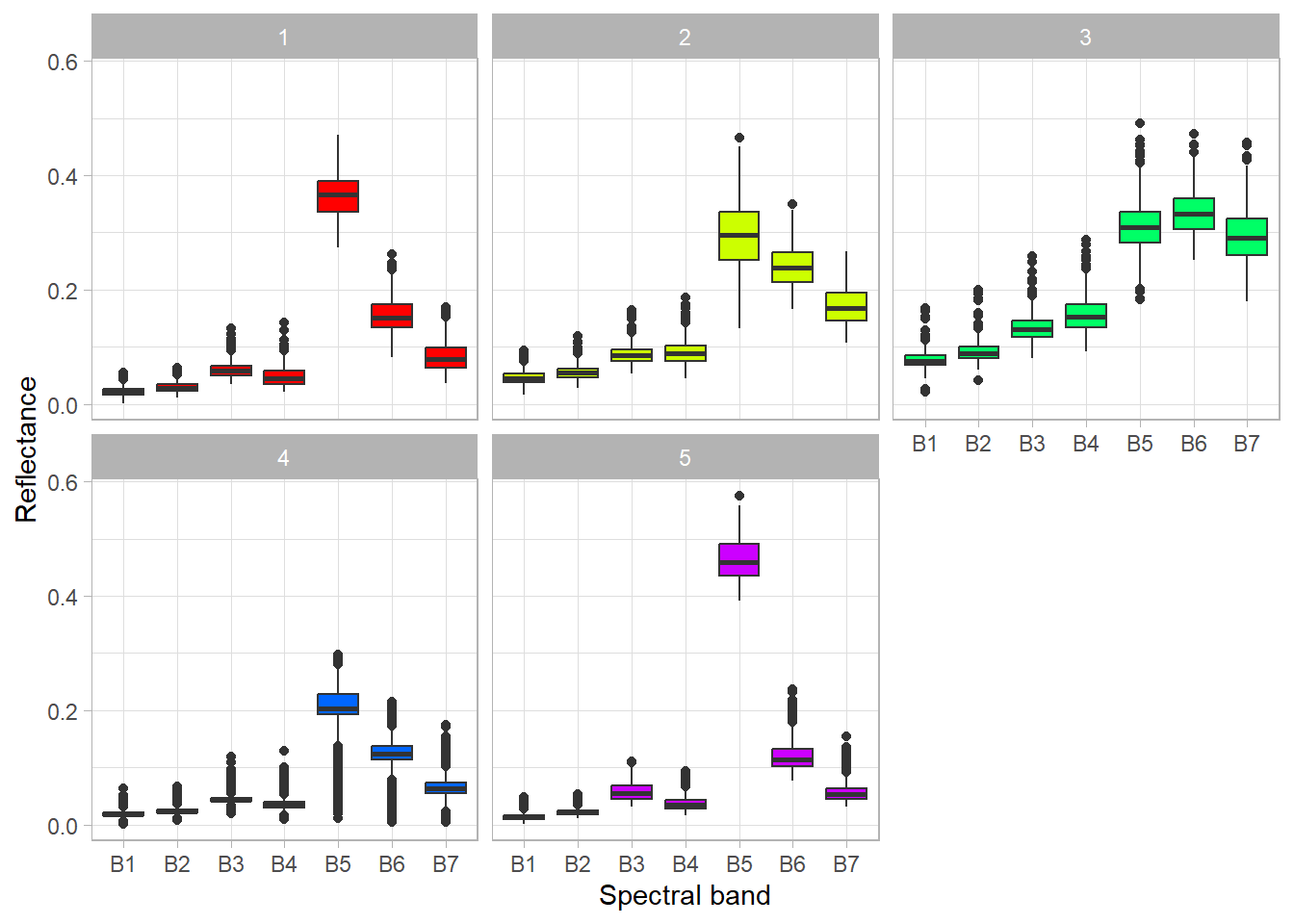
ggplot (stats, aes (x = band, y = value, fill = cluster)) + geom_boxplot (show.legend = FALSE ) + scale_fill_manual (values = colors) + facet_wrap (vars (cluster)) + xlab ("Spectral band" ) + ylab ("Reflectance" ) + theme_light ()
= rep (NA , ncell (landsat)) # prepare an empty vector complete.cases (mat)] = mdl$ cluster # assign clusters to vector if not NA = rast (landsat, nlyrs = 1 , vals = vec) # create raster
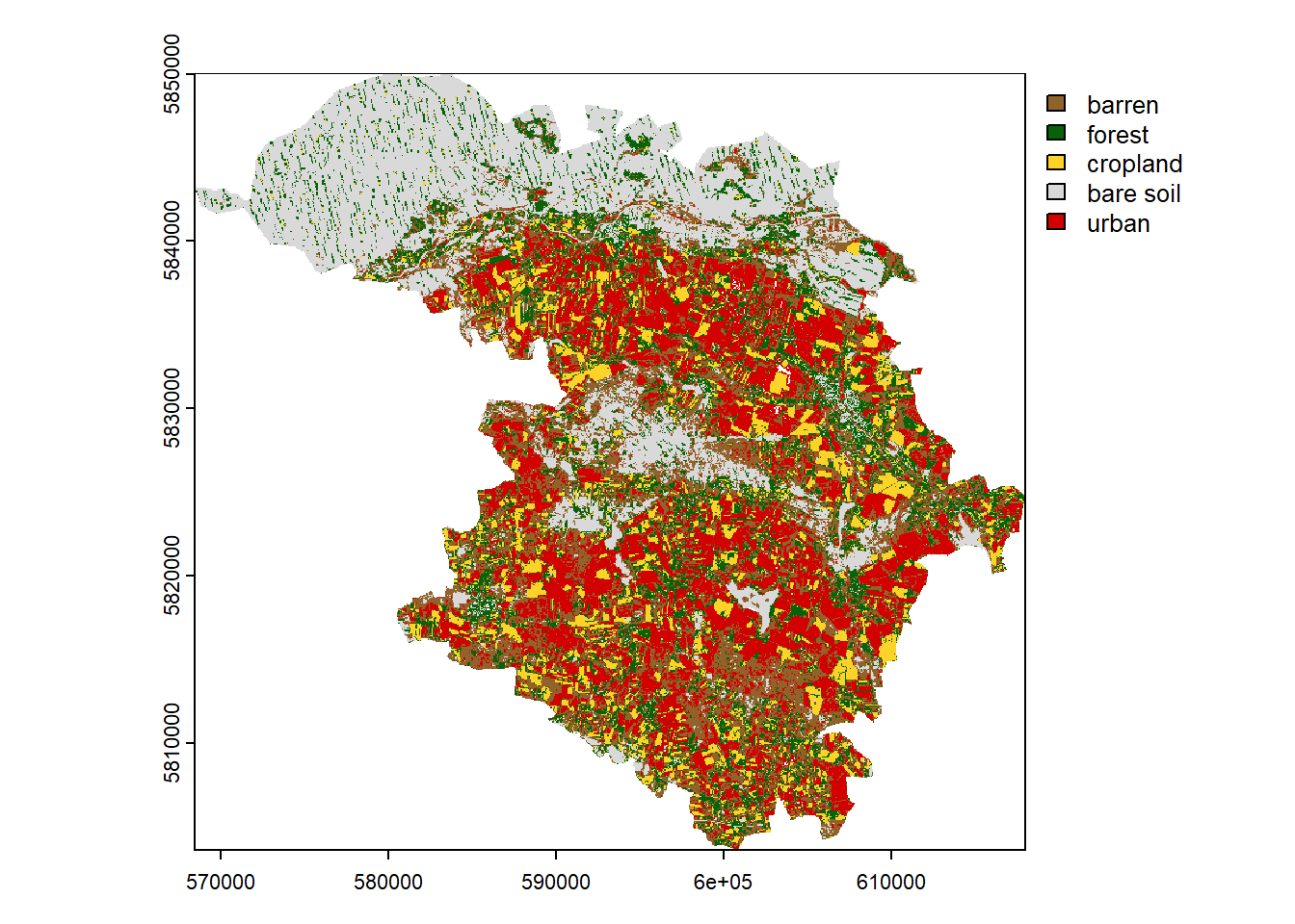
Present the results on a map and choose the appropriate color scheme.
= c ("#91632b" , "#086209" , "#fdd327" , "#d9d9d9" , "#d20000" )= c ("barren" , "forest" , "cropland" , "bare soil" , "urban" )= plot (clustering, col = colors, type = "classes" , levels = category)